This is me playing chess against SO-101, a cheap 6-DoF robot arm, controlled by a finetuned π0.5 VLA model. After I make a move, a small CNN detects the change, calls Stockfish, after which the VLA actually performs the physical move. This is a short informal description of the setup and where we plan to take it next.
Hardware Setup
The whole setup costs about $360, excluding the Raspberry Pi (which I already had). There are two SO-101 arms: a follower arm that actually plays, and a leader arm that I move by hand when recording demonstrations for behavior cloning. The difference is that the leader’s servos are geared lighter so that it’s easy to backdrive. There are two cameras: one on the wrist and one overhead, on a printed stand. The servos report back their position and current draw.
This is where I got the parts:
| Part | Link | Price |
|---|---|---|
| SO-ARM101 Servo Motor Kit Pro (both arms) | Mouser | $270 |
| SO-ARM101 3D Printed Skeleton (both arms) | Mouser | $40 |
| 2x innomaker 1080p camera (wrist + overhead) | Amazon | $21 each |
| Raspberry Pi 4 | already had one | |
| printed overhead camera stand | GitHub | ~free |
And the building process:
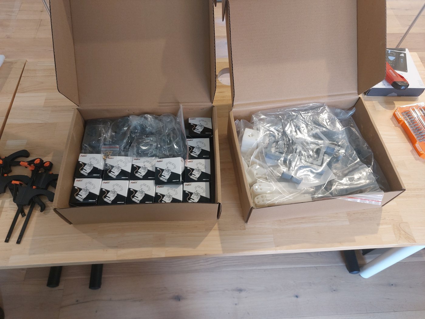
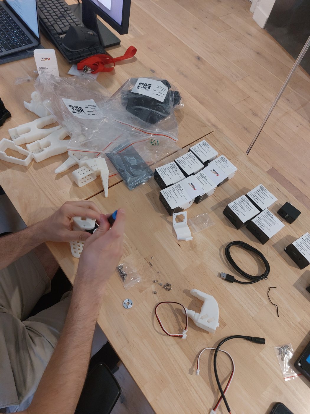


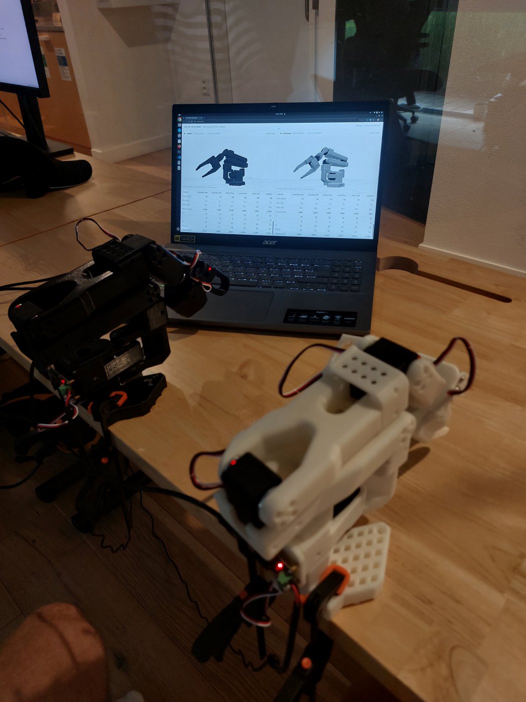
The first thing I did with them was a simple pick-and-place task to test everything: Fine-tune SmolVLA1 on 50 teleoperated demonstrations of moving a tape onto a marked cross. It worked surprisingly robustly for such a small number of demonstrations:
Software Setup
For the actual chess playing task, I fine-tune π0.52. It’s served on a GPU in the cloud, connected with the arm via my laptop and the Raspberry Pi (used only for convenience, since the whole setup is 4 USB cables). When experimenting with simulation, the simulation host exposes the same HTTP interface as the Raspberry Pi, so it’s fully transparent for the rest of the code.
Data Collection
The model learns from a corpus of demonstrations showing how to actually move the pieces. First, the demonstrations are collected simply by me performing the movement using the leader arm (video on the left). Once the robot is capable enough, I let it perform the movement by itself, and I only take over control when it starts to go wrong (video on the right).
I use Magnus Carlsen’s games during the collection, to stay as in-distribution as possible for when I play (haha). The pieces, squares and clutter around the target are therefore distributed the way an actual game distributes them.
During coaching, I also grade each episode as success, success but mispositioned, or failure. For the demo above, I then trained on all the frames from human take-over, plus all the frames from successful episodes.
The datasets might be useful even for someone else, and they are on Huggingface Hub: king-only moves (250 episodes of the single-piece task), human demos (567), hard human demos (281), and coached (166, with grades and per-frame policy or human tags).
Observations and actions
The policy’s observations consist of:
| observation | description |
|---|---|
| wrist image | 1280x720 RGB, undistorted, cropped |
| overhead image | 1280x720 RGB, undistorted, cropped |
| robot state | 6 joint angles, plus the gripper’s current draw |
| task string | “Pick up the pawn from g7” |
Both the overhead and wrist images are cropped outside of the chessboard (with some margin), so that the model is not distracted by the changing scene around the robot (e.g. a human opponent trying to confuse it). The wrist crop mask is recomputed every frame from the arm position (computed with forward kinematics) and the known chessboard position. Also, both images are undistorted to remove the terrible barrel distortion of the cheap cameras. I’m not sure this helped anything, but it might help us down the road when we pre-train in simulation (where the camera is not distorted at all).
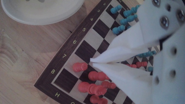
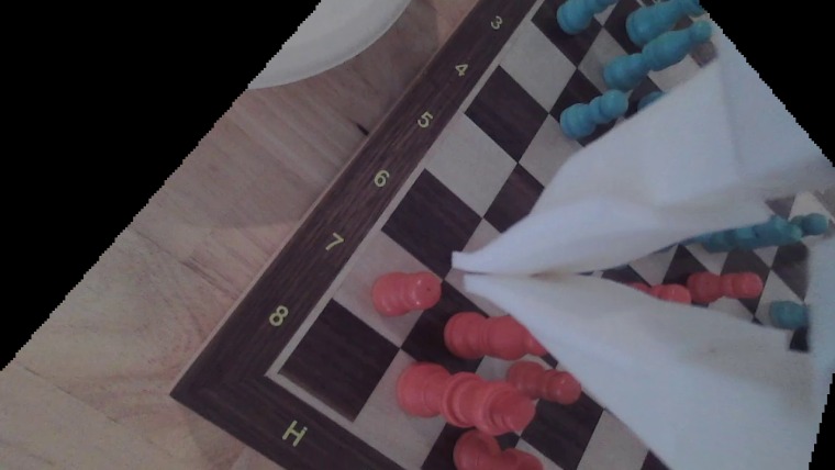
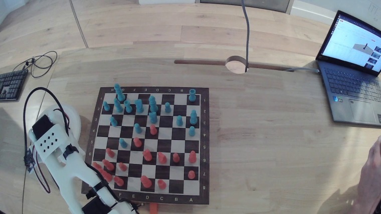
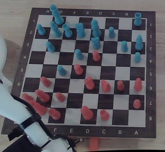
The gripper current is included because it unambiguously conveys the information of whether the gripper is currently holding a piece. It is fed to the policy as log(1 + mA). Whether it actually improves the policy is not yet measured.
The action is then simply the 6 absolute joint targets.3
Moving a Single Piece
The first version was just moving the king on an empty board, to get a sense of how many demonstrations we need for the model to learn to locate the squares by their names, and to perform the move. The video below is π0.5 fine-tuned on 250 human demonstrations:
When trying to make this work, I think it helped to unfreeze the VLM backbone instead of fine-tuning only the action expert (by default, lerobot keeps the VLM part frozen). Again, I need to properly measure this in the future.
Real-time chunking
Now is a good time to talk about Real-Time Chunking (RTC)4. The VLA’s action expert outputs chunks of 50 actions, so e.g. at 50Hz one chunk takes 1s to execute. The simple synchronous approach is to execute the current chunk, then ask for the next one, wait, and repeat. However, since the model inference roundtrip is ~600ms, this results in laggy motion.
The obvious fix is asynchronous inference, where we start computing the next chunk while the current one is still executing. However, since the state develops between when the next chunk inference is started and when it finishes, we need to make sure that the two chunks fit together, ie., that switching from one to the other doesn’t create a big jump. For example, if there are two possible ways to proceed forward from the current state, it could happen that the next chunk chooses a different one than the current chunk already committed to.
RTC is a principled way to do this - fix the actions that we already committed to (ie., the ones that will be executed before the next action chunk is ready), and inpaint the rest, while softly nudging the in-between actions so that the transition is smooth. The RTC paper contains the precise algorithm and pictures that explain it better than my hand-waving.
The laggy motion resulting from turning RTC off is shown in the video below on the left. However, it turns out that RTC also solves another issue, specifically the fact that the policy has no memory. This is a problem because the task is not fully observable - when approaching the piece, there is a moment when the wrist camera doesn’t see the board yet, but the overhead camera already has the relevant part of the board occluded by the arm. In that instance, the stateless policy has no way of knowing whether it’s approaching the piece or already returning home. This sometimes results in the robot being unsure what to do, shown in the video on the right.
The issue on the right occurred before I started using RTC. I fixed it by conditioning the model on the last 4 actions in addition to the current state, but all of that became unnecessary with RTC.
Validation metrics
Another interesting point is what metrics to look at when comparing checkpoints trained with behavior cloning. First I used validation loss, but for a flow model this doesn’t necessarily capture how well we model the joint actions or the end effector position. Instead, on the validation set, I now run the denoising plus forward kinematics and compute mean absolute distance between the predicted and gold gripper fingertip position.
The Full Chess Setup
Playing a full chess game is harder because, annoyingly, there are other pieces on the board beside the one we are trying to move. Also, there is taking pieces, castling, and en passant. And, we need to somehow decide which move to actually make, which involves detecting the board state and calling Stockfish.
Phase decomposition
To get a demo to work as fast as possible, I simplified a lot by splitting the move into phases and performing the easy ones with classic IK-based control, using the learned policy only for subtasks that actually require it. The phases are:
| phase | run by |
|---|---|
| hover over the source square | IK |
| pick | π0.5 |
| transport to the target square | IK |
| place | π0.5 |
| move home | IK |
The IK control assumes we know the position of the chessboard, so for now we just make the position fixed. With these simplifications, a lot of issues disappear. Of course, the smaller tasks are just simpler to learn, as the model does not need to understand where e.g. g7 is. But since we can compose any combination of phases, we also get castling and taking pieces for free. For example, when taking a piece, we just inject another IK-based phase moving the arm over a bowl beside the chessboard and releasing the gripper. The only tasks that really require precise visual-conditioned control are the picking up and placing down of pieces. One issue this introduces is that we need to know when a policy-controlled phase is finished, ie. when we should transition to the next one, but simple hard-coded heuristics work surprisingly well (gripper is closed/open and back at hover height, and it has already previously descended by at least 3cm).
One final advantage of the phased setup is that now the task is fully observable, so the robot never gets stuck not knowing whether it’s starting or finishing the episode. The end-to-end setup is more interesting as a real benchmark though, and we’ll return to it in the future.
Board state detection
We could leave the decision of what move to play to the fine-tuned π0.5, but that seemed like a big ask. So for now, we delegate it to Stockfish, meaning that we need some way to detect which pieces are where. A person looking at a frame from the overhead camera can read the position reliably. However, even frontier models cannot – I tried Opus 4.8, Gemini 3.1 Pro, and GPT-5.6 on a random position, and none of them got it remotely correct. I thought about buying a second overhead camera, or even about capturing frames from the wrist camera at different positions (by moving the arm in a scripted pattern), but it seemed like an overkill for now.
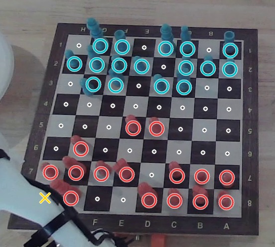
So again, I went with a simplified setup, where we only detect the position and color of pieces, but not their type, which simplifies it by a lot. During a game, we know the starting position, so if we can reliably detect which piece(s) disappeared and which appeared, we can infer the move. In the end, this worked very reliably.
The simplified detection is done via a small CNN (30k params) run separately for each square. As input it receives a 48x48 crop of that square (remember that we know the board position and the arm position), and it classifies the square as empty, black, white, or occluded by the arm (the actual physical colors of the pieces are orange and teal). The crop includes the square and also some neighborhood of it, since pieces mostly overflow to the square one up. I could directly train it with a few Claude Code prompts, since the training data could be extracted from the dataset of human demonstrations that I already collected (again, during the dataset collection I start with the initial chess position and each move is recorded), giving me ~72k data points. Here is what the detection looks like:

Control and Calibration
Control loops
There are four control loops running on top of each other:
| loop | rate | what it does |
|---|---|---|
| policy | ~2 Hz | predicts the next 50 actions (10 of them used) |
| chunk executor | 15 Hz | sends the next target from the chunk to the Pi |
| interpolator | 60 Hz | interpolates between consecutive targets (otherwise the motion is jerky) |
| servo controller | ~1 kHz | each servo runs its own PID |
Camera calibration
Both cameras are cheap USB camera modules with a wide lens, and they distort the image heavily. This might have turned out not to be an issue at all, but when I first saw it, I wanted to un-distort the images, just to make it easier for the VLA. Un-distorting also has two other advantages: It brings the observations closer to what is seen in simulation (useful in the future), and it enables the hacks we are doing now such as cropping cells from the pixels for pieces detection.
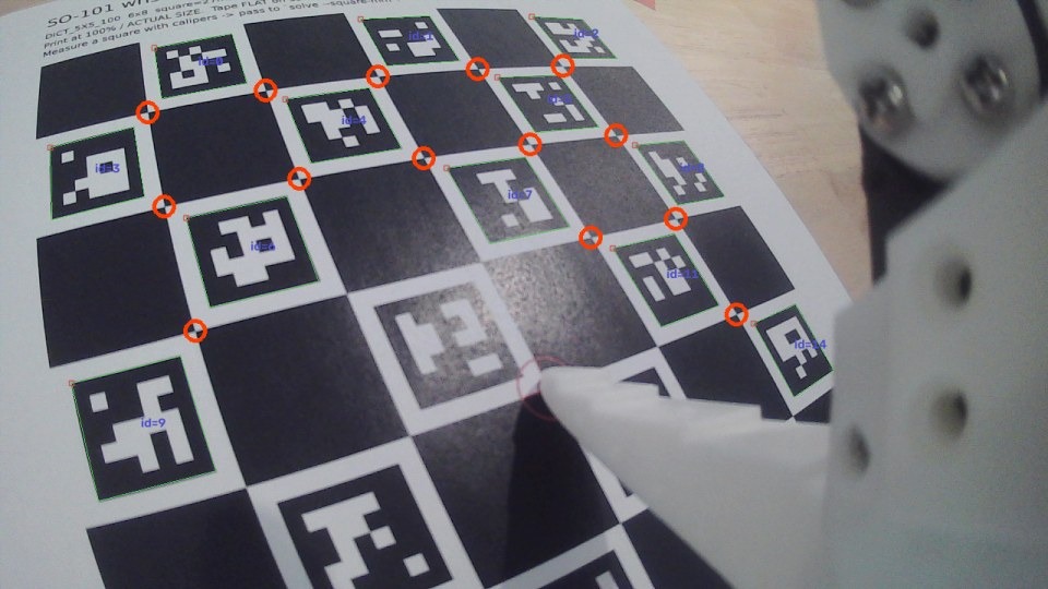
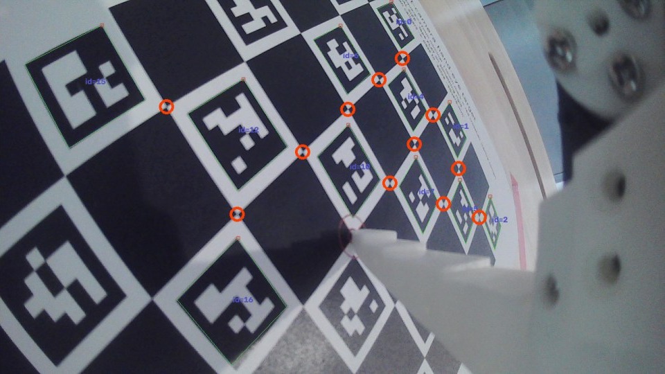
For the un-distortion I first needed to measure the distortion parameters (the camera’s intrinsic parameters). This is done by photographing a ChArUco board5 from many different angles (and prompting Claude Code to call the right OpenCV functions..).
In a second phase, I also calibrated the camera’s extrinsic parameters, ie. its position and orientation.
Again, this will be useful once we train in simulation, but also immediately now to allow e.g. cropping the observations around the chessboard.
This can’t really be measured with a ruler, because the camera’s optical center sits somewhere inside the housing.
So instead it is fitted from photos.
I tape the ChArUco board onto the table and move the arm to several poses, photographing the board at each one.
For every pose we know two things: where the gripper is, from the joint angles, and where the camera is relative to the board, from the photograph.
The unknown is how the camera is mounted on the gripper, and that one transform has to fit every pose at once.
Solving for it is a standard problem with a standard OpenCV routine (calibrateHandEye).
Ongoing Work
Besides simple behavior cloning on human demonstrations, I tried two interesting approaches: RECAP-style advantage conditioning, and training in simulation.
Advantage-conditioned behavior cloning
Pure behavior cloning has two problems: First, it assumes that all my demonstrated actions are worth copying, which is not true, because the way I move the arm is definitely not optimal. Second, when I then transition from manual collection to coaching, all the failed episodes are discarded instead of being used as negative examples for training.
RECAP6 instead learns a model of both good and bad actions. First, it trains a value function, a model that looks at one frame and predicts how much longer the robot still needs before the task is completed, with a failure counting as a large fixed penalty on top. I used a frozen SmolVLM2-500M with a small trainable head, trained on the episodes recorded during coaching. Every frame in the dataset is then scored by an n-step advantage: look 10 ticks ahead, and ask whether the value rose by more than the time those ticks cost. The best 30% of frames by this score are labeled positive and the rest negative. The label is only text, " Advantage: positive" or " Advantage: negative" appended to the task string, and the policy trains on all the frames.
During inference, we could simply ask for a “positive” action. Instead, RECAP uses classifier-free guidance (CFG), which means we ask for a positive action and also a neutral action (ie. one without conditioning on the advantage), and push the action in the direction from the unconditioned prediction to the positive one (how far we push is a hyperparameter). To enable the unconditioned prediction, 30% of frames train with no advantage suffix at all.
Training in simulation
I also tried training purely in simulation – used SAM3D for getting 3D models of the pieces (the precise dimensions needed some rescaling afterwards), measured the cell size, the board position, etc., and then Claude Code wrote an IK-based expert that was able to correctly move the piece most of the time. The successful expert trajectories were then distilled via behavior cloning into the VLA. The idea of the distillation is that the expert uses privileged information from the simulator, such as the precise position and orientation of the piece, which is then not available in reality. I used Isaac Sim first, but the tooling seemed a bit heavy and cumbersome, so I switched to Maniskill for the experiments that I did. Now I think I’ll switch to MJWrap, since MuJoCo is just so much more standard.
After training in simulation, π0.5 got a nice score in simulation, but was terrible in reality, which is to be expected. I decided not to push this before the demo was done, but pre-training in simulation is right now my main focus.
Discarded Idea: Simplifying Reality
One idea I really liked at the beginning was: Rather than making the simulation more realistic, make reality simpler. I thought this basically solves the sim2real gap. Instead of giving the simulator the real board’s colors and geometry, keep the render as trivial as possible, flat and unlit with the arm rendered as a plain silhouette, and filter the real camera stream down to that same look before the policy sees it. We can then do other interesting stuff like directly painting the information about the source and target squares into the observations, sort of an “augmented reality” for the policy. This is what I pictured it to look like:
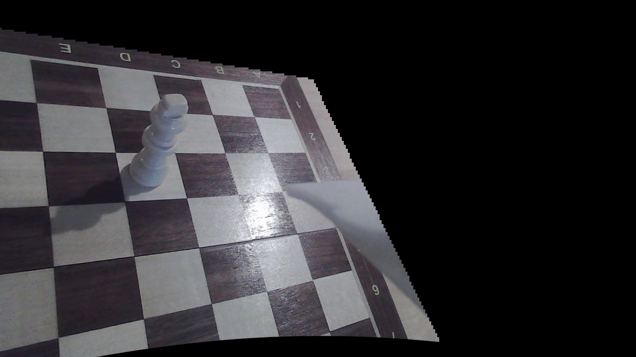

But this never worked reliably. Turning a real frame into that flat look means deciding exactly which pixels constitute the piece, and also exactly where the chessboard is. Once we have that, we simply render the synthetic chessboard and filter out everything except of the piece pixels. However, even when I run SAM3 to segment the piece, it often failed, producing a weird mask of e.g. half of the piece – and we’d need something faster than SAM3. Also, figuring out exactly how the chessboard is positioned relative to the camera is not easy (even after we calibrated the camera position relative to the robot). Relying on forward kinematics is not precise enough for this cheap robot. And once the wrist is very close to the chessboard, it’s impossible to detect the chessboard position from the images.
I didn’t use this preprocessing for now. My working hypothesis is that the biggest sim2real issue is actually not the visual observations, but the hard-to-simulate dynamics of the cheap robot. And after all, this is not really the kind of stuff I should try right now – of course we might be able to simplify the training if we introduce more custom preprocessing or extract more privileged information, but that kind of goes against the point of experimenting with VLAs.
What’s Next
The robot can play chess, but all the design decisions were made based on vibe, without any real ablations. Next, I’m evaluating the different setups rigorously, e.g. various VLAs (SmolVLA, π0.5), various adaptation algorithms (pure BC, RECAP), and pre-training in simulation. I also switched back to the end-to-end setup, because that is a more interesting task.
SmolVLA: A Vision-Language-Action Model for Affordable and Efficient Robotics ↩︎
π0.5: a Vision-Language-Action Model with Open-World Generalization. ↩︎
The policy predicts a chunk of 50 steps at once, but only the first 10 are actually used. ↩︎
https://docs.opencv.org/4.6.0/df/d4a/tutorial_charuco_detection.html ↩︎
Introduced in π*0.6: a VLA That Learns From Experience. ↩︎